The idea
Mechanical earthquake-cycle models track stress and friction on a fault. Those quantities are hard to measure at the scales that matter, and there may be no unique mechanical model of a given fault. kes takes a macroscopic view instead, in the spirit of Carnot’s engine that works “independently of any mechanism” and Jaynes’ maximum entropy reasoning. It tracks one kinematic quantity, the geometric moment : fault area times average slip, in m³. It then asks what the least-committal earthquake sequence is that respects
- an approximate long-term balance between moment accumulated by tectonic loading and moment released by earthquakes and afterslip;
- three well-established empirical laws: Gutenberg–Richter magnitudes, magnitude–area scaling and Omori aftershock decay.
Where nothing else is known, choices are made by maximizing entropy (uncertainty).
The model has three parts:
- an earthquake rate set by the moment budget;
- maximum entropy earthquake locations;
- maximum entropy afterslip.
All three act on a fault discretized into small patches. In the examples here the fault is a vertical strike-slip fault 200 km long and 25 km deep.
Earthquake rate from the moment budget
Each patch stores a geometric moment deficit. It grows with tectonic loading and shrinks when the patch slips in an earthquake or in afterslip. Summed over the fault, the deficit is
the moment accumulated minus that released coseismically () and by afterslip (). The earthquake rate is proportional to this deficit, plus an Omori aftershock term:
The aftershock productivity grows with mainshock magnitude, (Reasenberg & Jones, 1989). The constant is the value that gives moment balance on average:
Here is the mean moment per earthquake under the Gutenberg–Richter distribution, and is the recurrence time of the largest event. A slow feedback nudges so that release keeps pace with loading.
The rate is accumulated rather than sampled. The running count produces an earthquake every time it passes a whole number, so the rate climbs steadily while the fault is quiet and drops after large releases. Each new earthquake is built in four steps:
- Draw a magnitude from a truncated Gutenberg–Richter distribution with slope .
- Convert it to a rupture area with , with in km² (Allen & Hayes, 2017).
- Grow a circular rupture around the centroid (described next), truncated at the fault edges.
- Assign slip that decays exponentially away from the centroid, with small random perturbations. Slip is capped so that no patch releases more moment than it has stored.
Runs start from a “spun-up” deficit, as if the fault had already been active for a long time.
Where earthquakes happen: maximum entropy
Where should an earthquake of magnitude be centred? With no information at all, the maximum entropy answer is “anywhere”: . kes adds three constraints:
- the probabilities sum to one;
- the expected logarithm of the stored moment at the centroid, , is fixed;
- that expectation can depend on magnitude.
Maximizing the entropy subject to these constraints gives a power law in the stored moment:
The exponent is the Lagrange multiplier of the moment constraint, written in the paper. It sets how selective an event is:
- With , the smallest earthquakes ignore the moment field and can occur anywhere.
- As grows, approaches (1.5 in the examples), and large earthquakes increasingly favour regions that have stored the most moment.
After a large earthquake, the same distance kernel used for afterslip (below) also raises the probability of nucleating near the rupture. These are aftershocks in space as well as in time.
Afterslip: maximum entropy again
After a large earthquake ( in the examples), patches that still hold residual moment can slip slowly. kes again seeks the least-committal distribution, this time for afterslip speed , constrained only by a finite mean speed. Maximizing the relative entropy gives an exponential distribution. Taking the residual moment as the driving potential gives afterslip that decays exponentially in time and releases exactly what is left.
Where afterslip happens is set by a spatial kernel that decays with the distance from the rupture, with km. The initial velocity is the product of three factors:
The second expression is the time evolution, which keeps . Here , because moment scales as length cubed (see Eq. 8 of the paper). Inside the rupture the kernel is large but most of the moment is already spent. Far away, moment is available but the kernel is small. So afterslip peaks in a halo just outside the rupture.
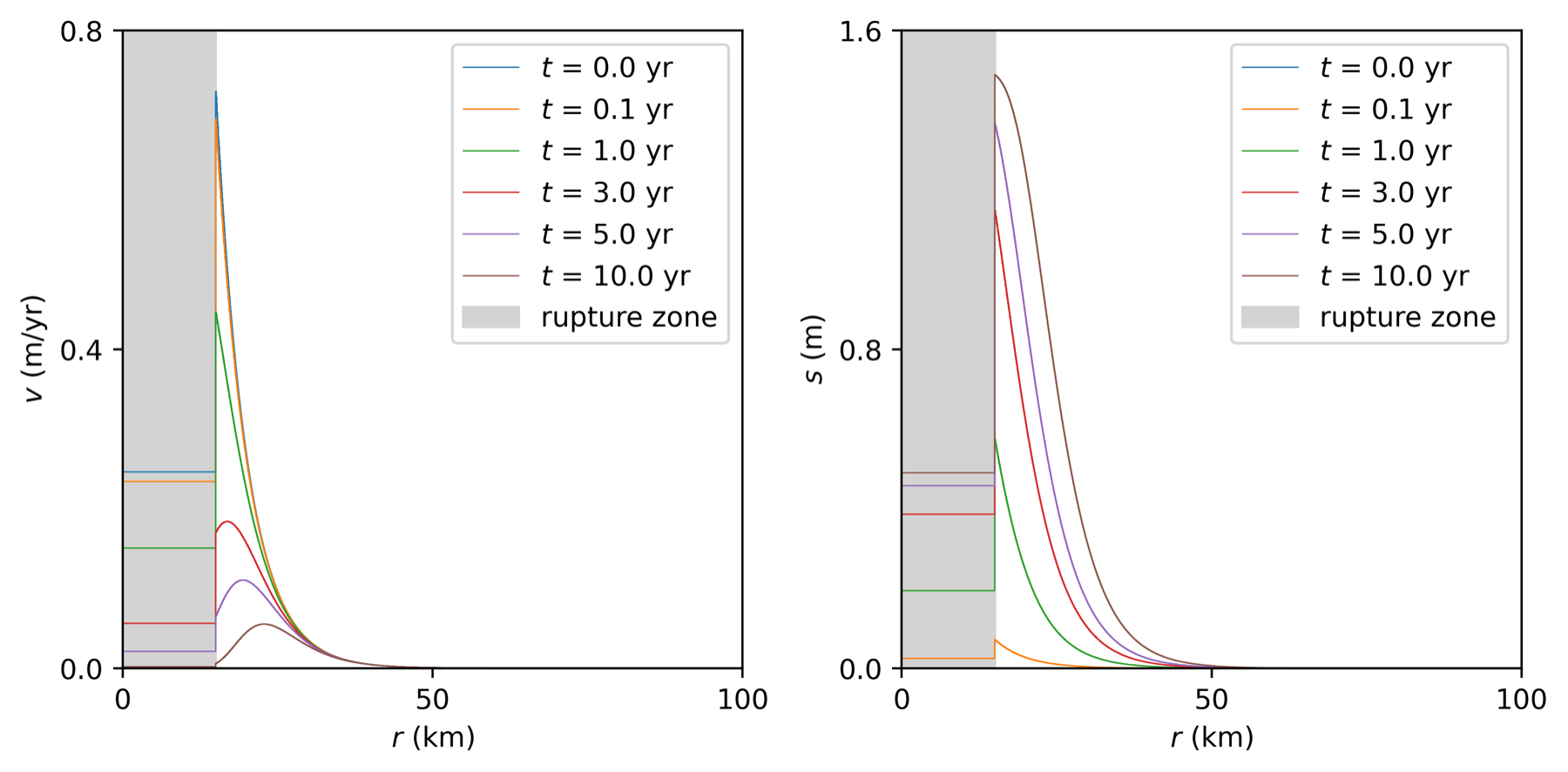
Afterslip velocity (left) and cumulative afterslip (right) against distance from the rupture centre, at six times after the earthquake. The gray band is the coseismic rupture. Velocities peak at the rupture edge, where the kernel and the residual moment are both large.
What a sequence looks like
The paper’s example is a 1,000-year run on 0.5 km × 0.5 km patches:
- loading of 10 mm/yr everywhere, plus a 20 mm/yr Gaussian “pulse” centred at km;
- and –8;
- Omori with a one-day offset;
- afterslip triggered by events.
It produced 1,272 earthquakes. Accumulation came to 97% of release, and afterslip accounted for 18% of the release.
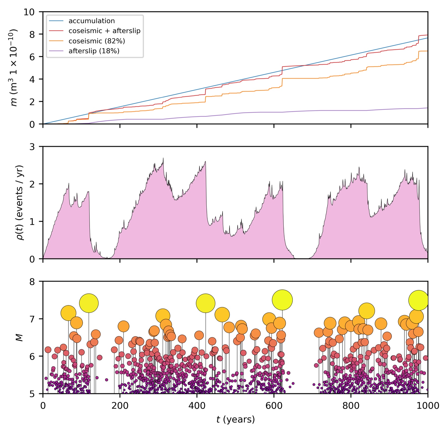
Top: cumulative geometric moment, comparing steady accumulation (blue) with coseismic (orange) and afterslip (purple) release. Middle: the earthquake rate . It climbs between large events and drops after them. Bottom: magnitudes. Clusters follow high-rate periods, and some (not all) large events are followed by decades of quiescence.
The fault-plane snapshots show the same run before, during and after an earthquake. In each pair, the upper panel is the moment released that year and the lower panel is the accumulated deficit.
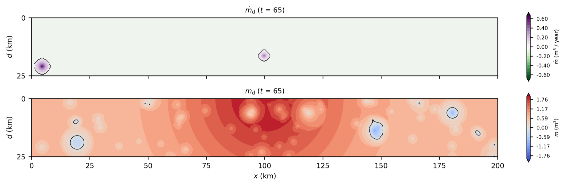
Before: the fault is broadly in deficit (red), most strongly over the loading pulse at –125 km. Small earthquakes show up as isolated purple specks.
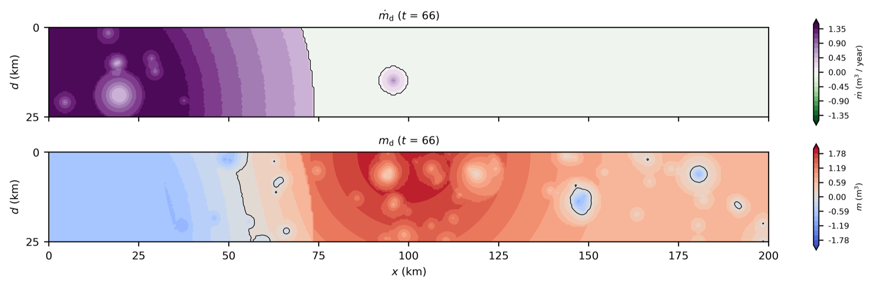
During: an earthquake releases moment over km (purple, upper), driving that region into local excess (blue, lower). Its aftershocks are the small circular patches nearby.
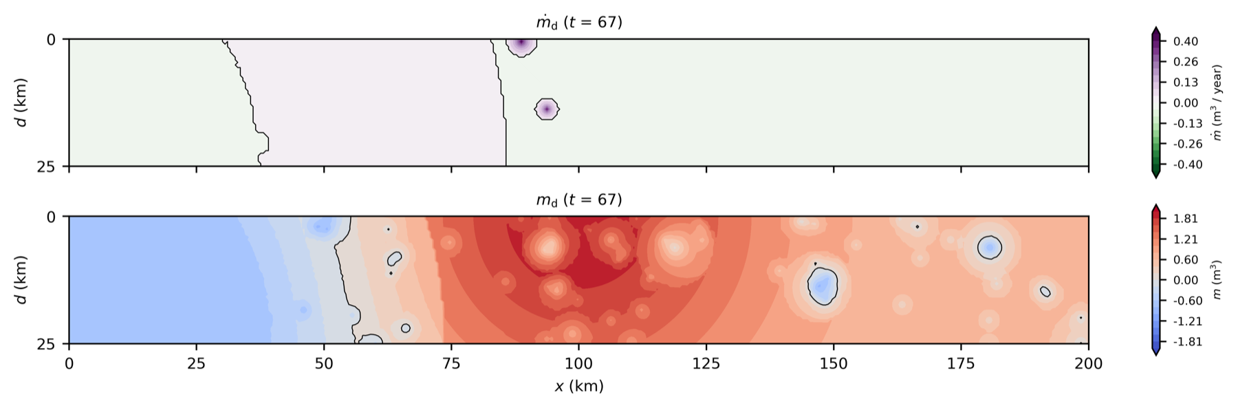
After: a band of afterslip between 30 and 85 km continues to release moment around the rupture.
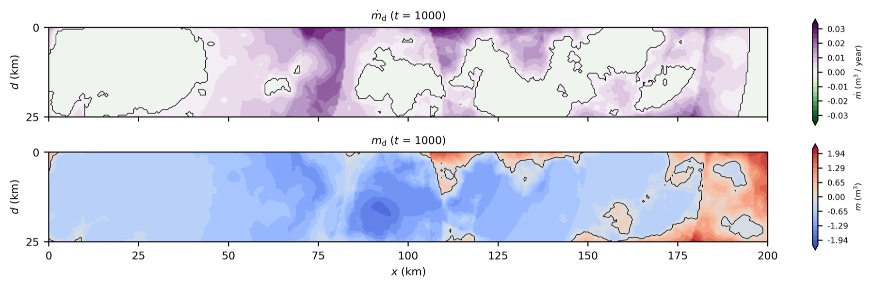
After 1,000 years, the history of ruptures has left a patchy deficit. The edges of old large ruptures remain visible near , 110 and 185 km.
Randomness versus loading
Because runs are cheap, kes can generate ensembles. Two experiments separate the effects of chance and of loading:
- Changing only the random seed produces qualitatively different histories. Event counts vary by about 35%, and long quiescent periods appear in some runs but not others.
- Shifting the loading pulse with the seed fixed changes the timing and number of events by less than 1%. The largest earthquakes move with the pulse.
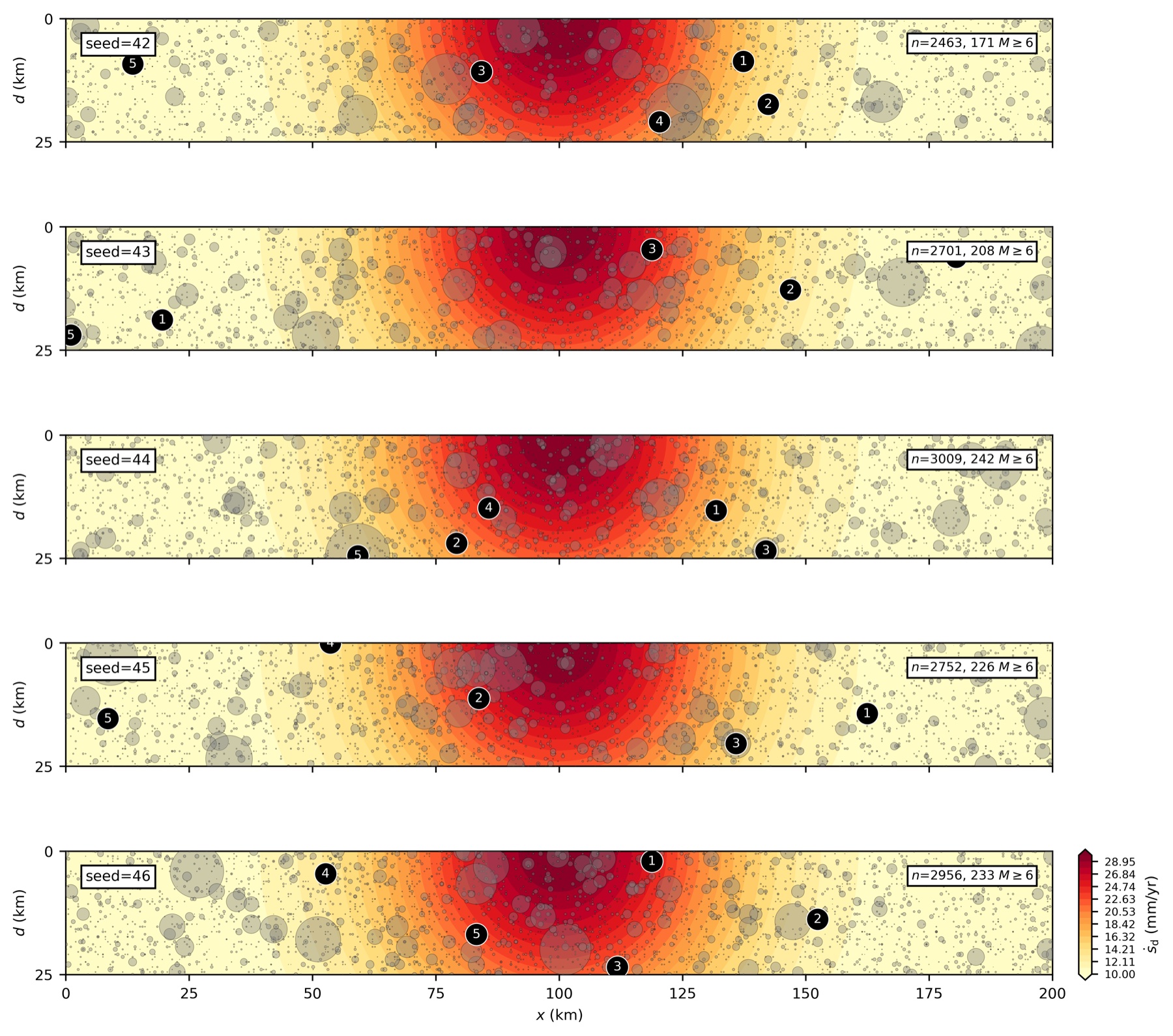
Centroids (gray, sized by magnitude) over the loading rate for five random seeds. The numbered discs are the first events. They differ from run to run, but cluster on the loading pulse.
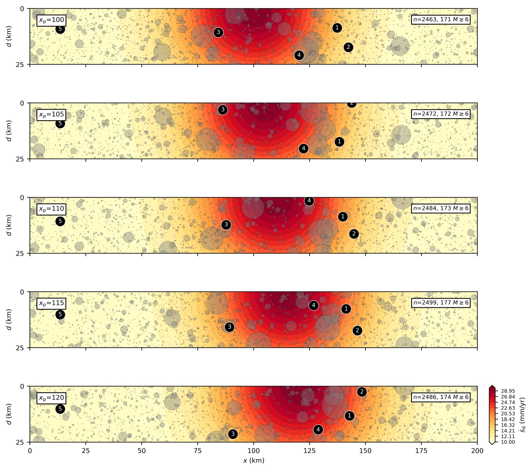
The same seed with the pulse moved from 100 to 120 km in 5 km steps. Most of the first large events track the pulse. One instead jumps between patches of similar stored moment.
Nothing in kes adjusts earthquake size, so the catalogs recover the prescribed -value. The Omori exponent comes out lower than prescribed, because the moment-budget rate briefly drops after large releases and then recovers as loading resumes.
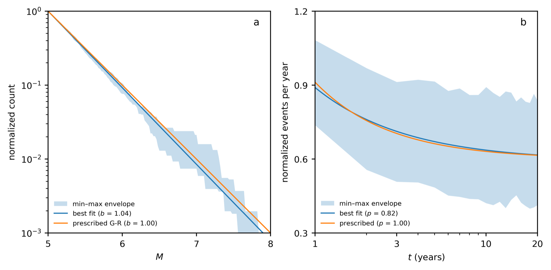
Prescribed (orange) and recovered (blue) statistics from the ensembles. Left: magnitude-frequency, with prescribed and recovered. Right: aftershock decay, with prescribed and recovered.
How kes differs from ETAS
kes uses the same Omori aftershock term as the widely used ETAS model, but differs from it in several ways:
- Driver. It tracks a moment field that is loaded tectonically and depleted by slip, rather than a self-exciting point process.
- Finite ruptures. Earthquakes are spatially extended, not point sources.
- Locations. Centroids are chosen from the current stored moment, not from kernels around past epicentres.
- Afterslip. Afterslip spends stored moment and so lowers local earthquake likelihood. It has no direct analogue in ETAS.
Together these produce behaviours a constant-background ETAS model does not: quasi-periodicity, semi-clustered large events and quiescent epochs.
The algorithm
- Compute the rate constant from the moment balance.
- For each time step:
- Release afterslip from earlier large earthquakes.
- Add tectonic loading.
- Compute the rate from the moment deficit and the Omori term.
- Accumulate , and emit one earthquake for each whole number passed.
- For each earthquake:
- Draw a magnitude.
- Choose a centroid from .
- Generate slip.
- Update the moment budget.
- Start afterslip if the earthquake is large enough.