A shadow, not a trigger
The on-fault page solves three rough faults that break the free surface at one load. The question behind it was whether the faults trigger one another: whether A’s slip brings B or C to failure before the remote load would. Measured on that system, it does not. For each fault the load at which it first slips is the same, to the bisection tolerance of 0.1 %, whether it is solved alone or in the system, with both P0 kernels: the remote load reaches an element’s strength before any neighbour’s stress does. What the neighbours change is completion. Solved alone, C has activated 73 % of its area by 1.6 λ₀; in the system, in A’s stress shadow, 28 %. A and B, which are fully active by 1.6 λ₀ either way, are behind by under 1 % at 1.1 λ₀. The two kernels agree on every number.
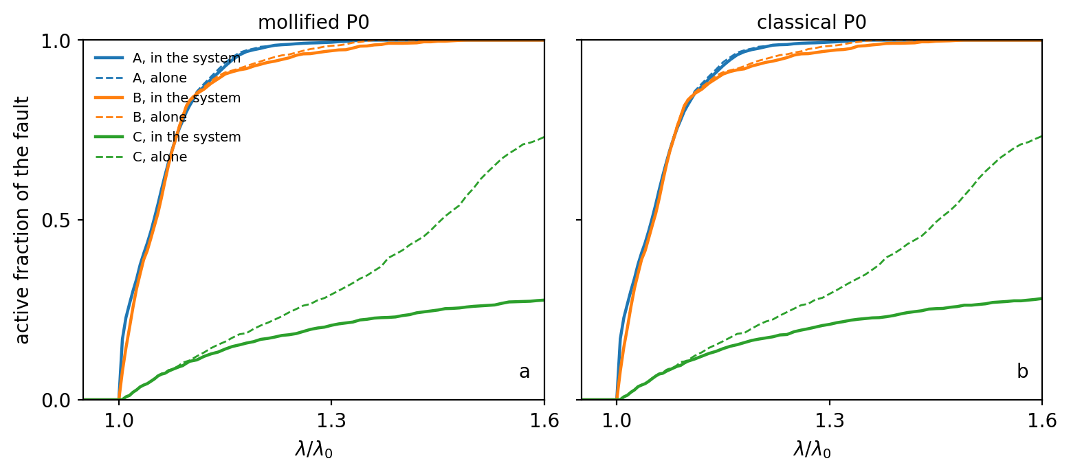
The failure-load scan on the three-fault system. Active fraction of each fault against the load λ in units of λ₀, the first failure with no interaction, solved alone (dashed) and in the system (solid), for a the mollified kernel with the free surface folded in and b the classical triangular dislocation. The onsets never move; the shadow acts on how far each fault goes.
That is a static result: the LCP at each load has one solution and no history. Local, positive transfer, one element’s slip bringing its neighbours to failure, is a different thing, and it needs no second fault.
One fault is the avalanche system
Take A alone, on the page’s own mesh (3748 elements of side h = 0.25 km once the junction constraint is gone), the same roughness, friction 0.6 on 150 MPa, the same thrust load, and run the loading history of the active fractal page on it: every element locked; the load rises until one element reaches its static strength; that element slips by exactly the amount that returns it to its dynamic strength, 10 % lower, and re-locks; its slip changes the stress on every other element through the interaction matrix; any element now at static strength slips too, and so on until the fault is in equilibrium again. One event is the difference between two equilibria. There is no time and nothing propagates; the load is a parameter.
The interaction matrix decides what this history can do. Its branching ratio, the stress one failure sends to the others as a fraction of the stress it sheds, is 0.98 on A, averaged over the elements. A near-planar crack under uniform load is critical by geometry: the interior row sums of its self-stress operator nearly vanish, because a dislocation loop that closes transfers everything it releases. The roughness, the rim and the free surface make up the missing 2 %.
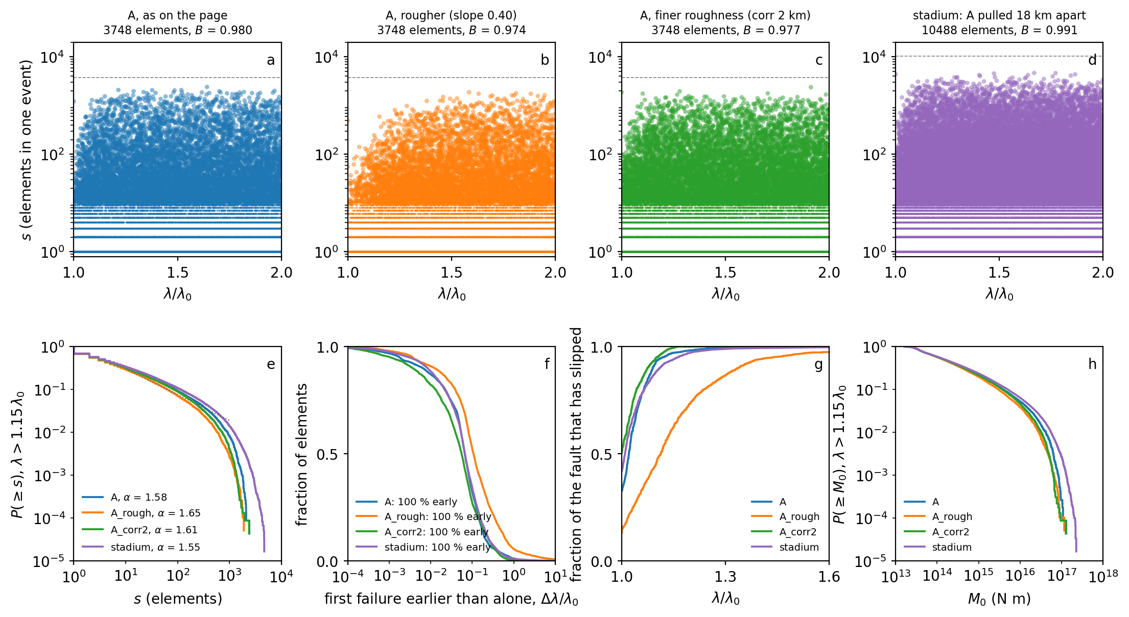
The loading history on one fault. a–d, the size of every event in elements against the load, for A as on the page, a rougher A, an A with finer roughness, and the stadium of the next section; the dashed line is the whole fault. e, the distribution of sizes once the history is steady (λ > 1.15 λ₀), with the maximum-likelihood exponent of each. f, for every element, how much earlier it first failed than the remote load alone would have failed it. g, the fraction of the fault that has slipped at least once. h, the moment distribution.
On A, 98 % of all element failures are transfer-triggered: of the 1.18 million failures to twice λ₀, only the 26,655 that start an event are the load’s. Every element fails earlier than the remote load alone would fail it, by a median of 0.07 λ₀ and a 90th percentile of 0.21 λ₀. The first event, at λ₀ itself, is the near-planar belt where the roughness tapers to zero at the rim and the trace, 1224 elements at once, a third of the fault. Past the transient the sizes are a power law: the maximum-likelihood exponent of the density, fitted above ten elements, is 1.59, the largest event covers 64 % of the fault, and events of a quarter of the fault or more recur 224 times in the history, spaced 0.0045 λ₀ apart on average with a coefficient of variation of 1.35, which is to say not periodically.
The resolution ladder
Every size above is in elements. The slip of one failure is the 9 MPa strength drop over the element’s self-stiffness, and that stiffness scales like 1/h, so an element fails more often on a finer mesh and the lower end of every distribution is set by the mesh. The ladder runs the same fault at h = 0.35, 0.25, 0.18 and 0.13 km with the mollification width at 0.1 h throughout and the taper belt held at the page’s 1.5 km in kilometres, not in h, so that the fault itself does not change between rungs.
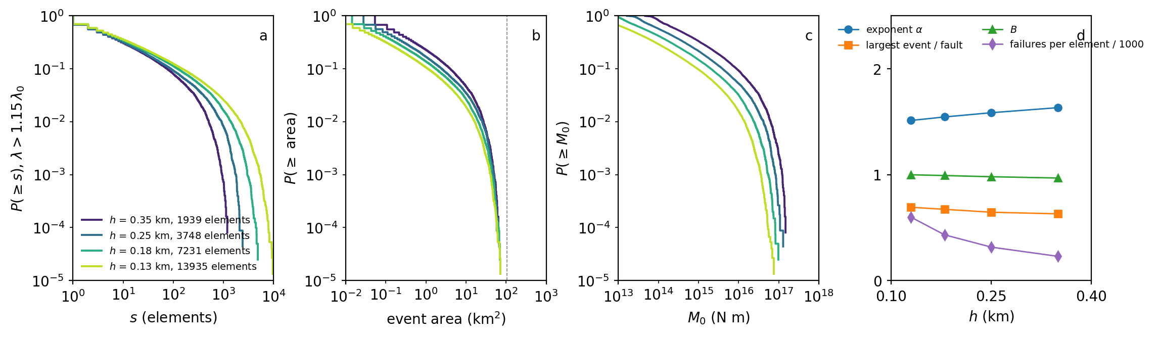
The same fault at four resolutions. a, event sizes in elements: the curves separate because the smallest event is one element. b, the same events by area: above a few square kilometres the curves collapse, and the dashed line is the fault. c, by moment, where they do not: each failure moves an element by the drop over a stiffness that scales like 1/h, so the moments scale with h. d, the exponent, the largest event, the branching ratio and the failures per element against h.
What belongs to the fault. The largest event is 63, 64, 67 and 69 % of the fault from the coarsest rung to the finest, and the size distribution by area is the same curve above a few square kilometres on all four. The transfer signature per element is resolution-independent: a median advance of 0.06 to 0.07 λ₀ and a 90th percentile of 0.21 to 0.22 λ₀ on every rung. The number of elements that fail per unit load scales exactly like 1/h (227, 315, 431, 597 failures per element to twice λ₀), as the stiffness argument says it must.
What moves with the mesh. The branching ratio climbs toward 1 with refinement, 0.968, 0.980, 0.991, 0.9986, because the row-sum deficit of a closed loop is an edge effect that refinement removes. The exponent drifts with it, 1.63, 1.59, 1.55, 1.51, toward the mean-field value of 1.5 that a critical branching process has at B = 1, and it is not converged at h = 0.13: the next rung would be a 35 GB matrix. The moments scale with h and are not fault properties at all in this model; a figure quoted in newton metres below is the h = 0.25 cell model’s. So the honest statement of the result is: a single rough fault is a critical system whose criticality sharpens with resolution, with events of up to two-thirds of the fault whose area distribution is converged, and an exponent between 1.5 and 1.6 whose exact value is still the mesh’s.
Roughness and length
The roughness sets the thresholds, not the criticality. A rougher A (rms facet slope 0.40 instead of 0.25) spreads the no-interaction failure loads of its elements from a 95th percentile of 1.4 λ₀ to 3.5 λ₀, and fifty of its elements can never fail under the remote load at all; the transfer brings those misoriented facets to failure anyway, a median of 0.11 λ₀ and a 90th percentile of 0.64 λ₀ early. Its branching ratio is 0.974 against 0.980, its exponent 1.65 against 1.59, its largest event 50 % of the fault against 64 %, and the fault-scale events fall from 224 to 66. Halving the correlation length to 2 km sits between the two: 131 fault-scale events, an exponent of 1.61. Roughness cuts the fault-scale events and spreads the first failures; it barely moves the branching ratio, because that is the geometry of a closed dislocation loop, not of its texture.
The stadium is A pulled apart along strike by an 18 km straight run, cut by the surface like A, with the same roughness, taper and gates: 10,488 elements, 290 km², a 27 km trace. Its branching ratio is 0.991. Its history has 70,168 events to twice λ₀, 7311 of them of a hundred elements or more, with an exponent of 1.55, closer to the mean-field 1.5 as the branching ratio approaches 1. The largest event is 45 % of the fault, 129 km², larger than all of A. What the stadium does not produce is along-strike ruptures: the events of a hundred elements or more have a median along-strike-to-down-dip aspect of 1.14, against 0.94 on the disc. The big events are compact patches that happen to sit on a longer fault.
Where the big events are
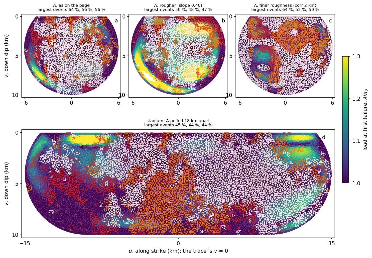
First failure and the largest events. Each fault in its own plane (u along strike, v down dip, the trace at v = 0), every element coloured by the load at which it first slipped, and the footprints of the three largest events of each history outlined in red, orange and white. a A, b the rougher A, c the finer roughness, d the stadium.
The first failures follow the roughness: the taper belt at λ₀, then the facets the remote load favours, then the ones the transfer reaches. The largest events are not the first-failing regions; they are the ones that have re-locked and been re-loaded by the slip around them, and on every variant they overlap the same part of the fault.
The same map without the drop
The history has two strengths per element: it fails at the static one and stops at the dynamic one, and that overshoot is what the neighbours feel. The static LCP of the thresholds scan has one. Its solution at a load is unique and path-free: every slipping element sits exactly at strength, every other below it, and the slip is a continuous function of the load, so there are no events to outline. What it does have is an activation load per element, the smallest load at which its slip becomes positive on a scan, and that is the counterpart of the first-failure map. Solved at the static strength and at the dynamic strength, the two LCPs bracket the history element by element: on A every one of the 3748 elements first fails no later than it activates in the LCP at static strength and no earlier than in the LCP at dynamic strength, and at twice λ₀ its slip lies between the two LCPs’ slips on every element.
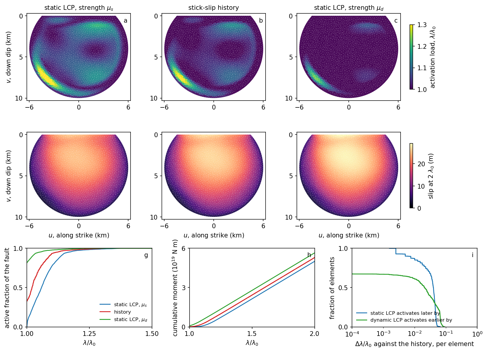
The history between the two LCPs, on A. a–c, the load at which each element first slips: in the static LCP at static strength, in the stick-slip history, and in the static LCP at dynamic strength. d–f, the slip at 2 λ₀ for the same three. g, the active fraction and h the cumulative moment against the load. i, per element, how much later the static-strength LCP activates it than the history does, and how much earlier the dynamic-strength LCP does.
| on A, to 2 λ₀ | LCP at μs | history | LCP at μd |
|---|---|---|---|
| activation load, median | 1.060 λ₀ | 1.021 λ₀ | 1.000 λ₀ |
| activation load, 90th percentile | 1.138 λ₀ | 1.090 λ₀ | 1.025 λ₀ |
| half the fault active | 1.060 λ₀ | 1.021 λ₀ | 1.000 λ₀ |
| 90 % of the fault active | 1.137 λ₀ | 1.090 λ₀ | 1.025 λ₀ |
| moment at 2 λ₀ | 5.00 × 10¹⁹ N m | 5.30 × 10¹⁹ N m | 5.65 × 10¹⁹ N m |
| mean slip of the active elements | 16.2 m | 17.1 m | 18.3 m |
| elements outside the bracket | 0 | 0 |
The three maps have the same shape because the geometry and the load decide where slip wants to be; the two thresholds decide when it arrives and in what pieces. The history’s first event takes the taper belt, 1224 elements, at λ₀ in one cascade; the static-strength LCP activates the same elements one by one between 1.0025 and 1.045 λ₀. In moment the history lands 46 % of the way from one LCP to the other. For a total at a given load, either LCP is within 6 % of the history and the pair bounds it. For the events, their sizes, their recurrence and who triggers whom, the LCP has nothing to say: all of that is the drop’s, and the drop is the one thing it does not have.
What this is, and is not
The moments are a cell model’s. Each failure moves one element by the drop over its self-stiffness, about 5 cm at h = 0.25 km, so an event over 64 % of A carries 1.3 × 10¹⁷ N m, a moment magnitude of 5.3, with an event-averaged stress drop of a fraction of a megapascal; the stadium’s largest reaches 2.2 × 10¹⁷ N m. Sizes as fractions of the fault, and the distributions by area and moment that the ladder shows to be resolution-independent, are the quantities to quote. The exponents carry the 5–7 % spread between update rules that the cascade solver measures on its own fixture (sequential, random and synchronous relaxation give different histories from the same state) on top of the drift with resolution above. A 2 % spread in the friction changes none of the numbers above materially (exponent 1.59, largest event 67 %); coupling the normal stress to the slip raises the branching ratio to 0.985 and the fault-scale count from 224 to 304, with the exponent at 1.57. On the stadium the symmetric part of the operator has a negative eigenvalue, the long fault’s body modes at this mollification width; the event-driven history never solves that system, only its columns, and the static solutions at the two strengths bracket every element the history activates, on every variant.
Reproducing it
python studies/active_fractal/onfault.py thresholds          # the opening figure
python studies/active_fractal/avalanche.py assemble A --workers 12
python studies/active_fractal/avalanche.py run A            # 3-5 s of history
python studies/active_fractal/avalanche.py run A --spread 0.02
python studies/active_fractal/avalanche.py run A --coupled
python studies/active_fractal/avalanche.py lcp A            # the static LCP's scan, ~15 min
python studies/active_fractal/avalanche.py figure            # the table, four figures
assemble is its own process because mhs parallelises over spawned
workers and a second pool after a closed one deadlocks; the matrix is
cached by the mesh’s hash and run reads it. The variants are A,
A_rough, A_corr2, stadium and the ladder A_h0.35, A_h0.18,
A_h0.13 (13,935 elements, an 8.7 GB matrix, 25 minutes on twelve
workers). The stadium is a spec key: run=18.0 on any fault of
system.build_system, gated in selfcheck.py -k system; the per-event
recorder is gated in -k slip.