loading…
The system and the meshes
The Taiwan Earthquake Model describes the island’s seismogenic structures as 66 surfaces. One of them, the Ryukyu–Nankai plate interface, is 2,000 km long and not a Taiwan fault, and it is left out; the other 65 are here, between longitudes 120.1° and 122.0° and latitudes 21.8° and 25.3°, in the frame of the Taiwan page: x east and y north in kilometres from the junction of the two Longitudinal Valley Fault segments, z up, the surface at zero. The system spans 194 km east–west and 393 km north–south and reaches 20 km down. Eight structures dip under 20°, the low-angle thrusts of the western foothills; seventeen dip between 20° and 45°; twenty-eight between 45° and 80°, the Longitudinal Valley Fault among them; and twelve are vertical. The largest is the 2,600 km² thrust of the west, the two Longitudinal Valley segments are the second and fifth, and the smallest has 54 elements.
The meshes are used as supplied, with a median edge of 1.85 km; one mollification width of a tenth of the median edge, 0.185 km, serves every structure, and the free surface is folded into the kernel as on the on-fault page. Three things about the facets had to be settled that the single fault never raised. The package takes the slip jump across each triangle’s vertex-order normal and builds its strike and dip frame from the same normal flipped upward, so a triangle wound downward has the sign of its own self-interaction reversed and the matrix is refused; every triangle is therefore wound upward, and on the twelve vertical structures, whose facets tilt a fraction of a degree either way, this makes the sign of the dip component of the painted rake a per-facet convention (the solve is unaffected: each element’s slip and traction live in its own frame). Forty-seven triangles of the low-angle thrusts lie entirely in the free surface, where the mesher laid the trace flat: slip there has no traction, their self-interaction is exactly zero and the complementarity problem would be singular, so they are dropped, 8 km² of 28,000. And the method has a resolution floor, the mollification width itself, which the supplied meshes go under in two ways: 572 slivers are thinner than it, down to 36 m² and 0.6 m of altitude, and 60 facets reach less than one width below the surface, among them a fan of one-degree triangles 10 m deep. The first assembled matrix kept them, and on exactly those facets the symmetrised operator was not positive definite (the next section says what that cost), so every facet thinner than the width or shallower than it is dropped: 579 triangles, 33 km², 0.12 % of the area, leaving 20,944. Twenty-nine buried triangles are exactly horizontal; on those the strike is east by convention and the painted rake means nothing.
What is swept
The tensors, the friction, the effective-stress models, the loads and the two slip rules are the Taiwan page’s, unchanged: the most compressive axis horizontal at seven azimuths from 90° to 150°, a regime from pure thrust to pure strike-slip in five steps, friction 0.6, an effective normal stress of 150 MPa everywhere or lithostatic minus a pore ratio of 0.4, and a scan from λ0, the load at which the best-oriented element of the whole system reaches its strength with no interaction, to six times it, under the fixed rake and the free one. One kernel, the Galerkin one of the Taiwan page, and here it is not a choice. The collocation operator, which drew the same map as the other two on the Longitudinal Valley Fault alone, is far from symmetric on the system: the smallest eigenvalue of its area-weighted symmetric part is −0.58 of the median diagonal, projected Gauss–Seidel grows its residual tenfold every eight sweeps on the thrust tensors, and the active-set solver cycles. The Galerkin operator is symmetric by construction and positive definite by the elastic energy argument wherever the quadrature resolves the smeared slip, which is what the resolution floor above enforces: with the sub-width facets in, a dense block of the operator on them had three negative eigenvalues and one free-rake scan ran away at 6 λ0; without them the full 41,888-square symmetric part has its smallest eigenvalue at +0.37, a hundredth of the median diagonal, measured by Lanczos. On that operator the fixed-rake problem is a strictly convex quadratic programme and the free-rake one a strongly convex cone problem, and projected Gauss–Seidel converges by theorem, so it is the only solver used. The matrix is 20,944 by 20,944 elements by three traction components by two slip components, 19.6 GiB, assembled once in sixteen hours on sixteen workers and shared by memory map between twelve, each of which takes one tensor’s scan of thirteen loads as a task: 140 scans, 1,820 solves.
What changes is that every element’s slip now loads every other element of the system, not only its own fault. A structure may be brought to failure by its neighbours’ slip before the regional load alone would do it, or held below failure in their shadow; the Taiwan page’s numbers for the Longitudinal Valley Fault alone are the control, and the figure’s last panel puts the two side by side. Where two structures pass within a mollification width of each other (18 pairs of element centroids, 312 within two and a half widths) the operator carries a slip mode of almost no energy, positive but soft, and that is where the largest slips and the slowest sweeps are.
What the sweep says
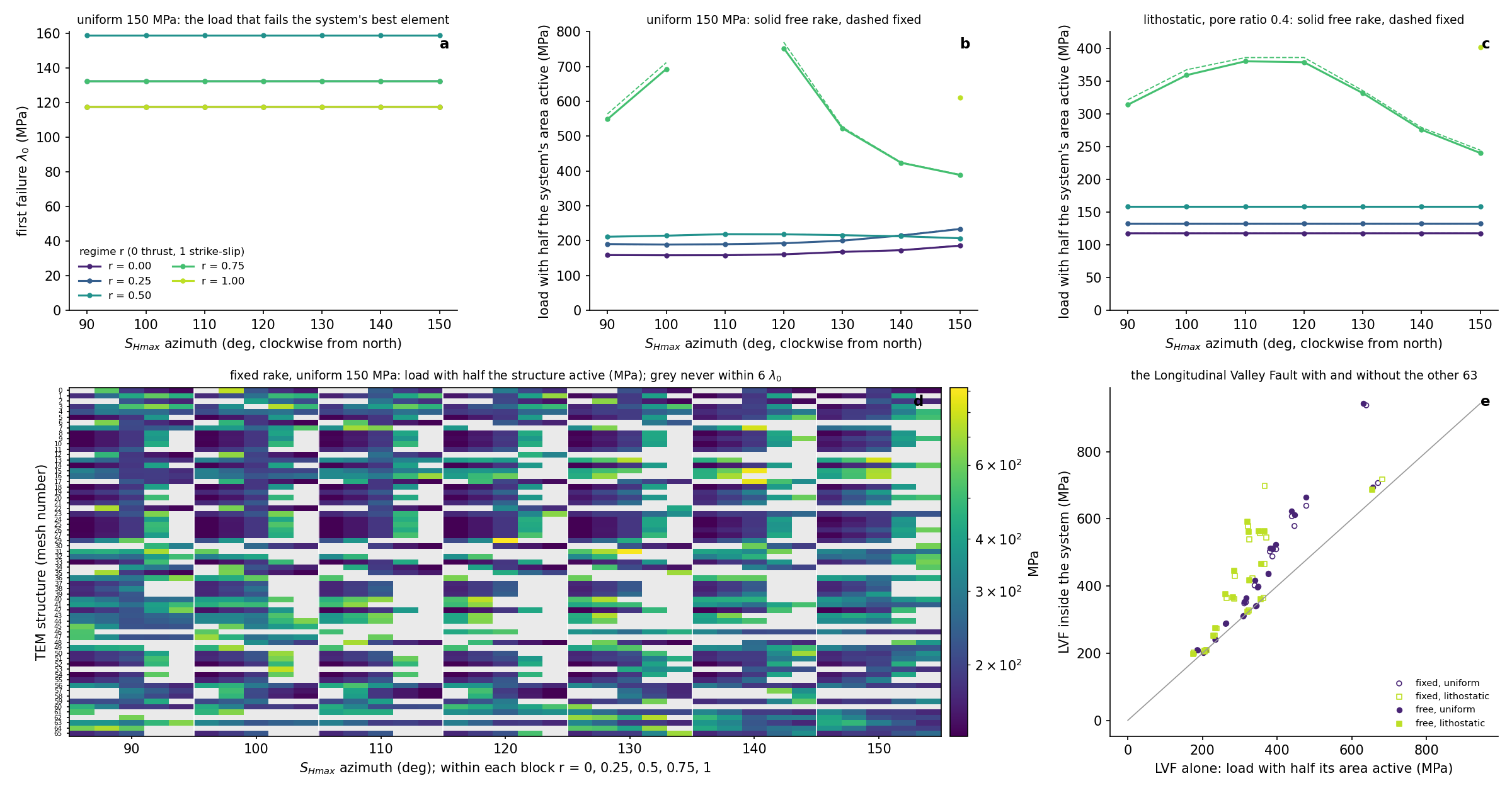
Every solve converged, by the solver the theorem covers. The 1,820 solves of the 140 scans all converged under projected Gauss–Seidel alone, none fell to a Newton step and none ran away: 255 sweeps per solve at the median and 867 at most, on the operator whose unreduced version had sent one free-rake scan to infinity. A fixed-rake scan of thirteen loads took ten minutes at the median, a free-rake scan 1.7 hours; 110 processor-hours in all, ten hours of wall clock on twelve workers sharing the matrix.
The system is not choosy about azimuth; the single fault was. On the Taiwan page the fault-normal thrust was the hardest tensor and the oblique strike-slip the easiest, a factor of 2.5 apart. With 65 structures at every strike and dip something is always well oriented, and the load at which half of the system’s area slips depends on the regime and barely on the azimuth: 158–186 MPa for the thrust tensor, 188–234 at r = 0.25, 207–219 at r = 0.5, which is 1.3–1.8 times λ0 throughout (panel b). The strike-slip-like tensors see a different system: at r = 0.75 half the area is reached only between 390 and 770 MPa and at azimuth 110 not at all, and the pure strike-slip tensor reaches it only at azimuth 150, at 623 MPa. At three times λ0 the thrust-like tensors have 67–85 % of the area slipping and the strike-slip tensor 17–37 %; by six times, 84 % at the median and never more than 92 %, so under every tensor a tenth of the system is misoriented or shadowed. Under the lithostatic model the shallow rows are so weak that half the area is already slipping at the uniform model’s λ0 for every thrust-like tensor (panel c): there the quoted load is λ0 itself.
Who carries the moment. Under the fault-normal thrust at azimuth 110 the low-angle thrusts of the west take it: structure 55 alone carries 23 % of the moment at 3 λ0, 50 another 14 %, then 19, 23 and 10, and the Longitudinal Valley Fault none at all. Under the strike-slip tensor at the same azimuth the vertical and steep structures of the north take over, 63 with 18 %, then 22, 48 and 57, and the Longitudinal Valley Fault 0.7 %. Only under the strike-slip tensor at azimuth 150 does the Longitudinal Valley Fault lead, 24 % of the moment, with 61, the long north-striking structure beside it, at 23 %. In the heat map (panel d) three structures are half active under every tensor and none stays grey under all of them; the earliest at the median over tensors are 8, 24, 27 and 18 at about 170 MPa, the latest 36, 31, 40, 49 and 41, the northern half of the Longitudinal Valley Fault, at 410–440.
The system makes the Longitudinal Valley Fault harder, never easier. Panel e puts the fault’s half-active load inside the system against its load alone on the Taiwan page, tensor by tensor. Every point lies on or above the line: the ratio is 1.14 at the median under the uniform model and 1.27 under the lithostatic, 1.47 and 1.90 at most, and at three times λ0 the fault’s active fraction is 0.27 inside the system at the median against 0.37 alone, lower by up to 0.30 and never higher by more than 0.001. The structures that fail first, at 135–185 MPa against the fault’s own 190–480, unload it: this is the stress shadow of the whole-system solve, larger than anything the single-fault page could show. (The alone values are the Taiwan page’s collocation kernel, whose Galerkin values differ by 2 %; the comparison is good to that.)
The free rake adds moment, not area, as on the single fault. Letting the slip direction go moves the half-active loads by at most 3 % and the active fraction at 3 λ0 by at most 0.015, and rotates the slip by 2 degrees at the area-median and 7 at the 90th percentile (2.4 and 9 under the lithostatic model). The moment rises by 9 % at the median, least (3 %) at r = 0.75 and azimuth 110 and most (17–27 %) for the pure thrust, which is oblique to much of the system: the rake is the tensor’s, and the free rule lets the obliquely loaded structures slip a little further along it.
Magnitudes, and the floor. Three times λ0 is a static load of 350–480 MPa of maximum shear, so the slips are not earthquakes: 34 m at the median active element, 160 m at the 99th percentile and 257 m at most, on the interior of the 15° thrust 55, and up to a kilometre at six times λ0 under the free rake. The largest slips sit on full-width elements of the largest low-angle structure, not on slivers: the resolution floor took the collocation kernel’s 2 km slips on 40 m slivers with it. Against the unreduced system’s 80 completed fixed-rake scans, dropping the 579 sub-width facets, 0.12 % of the area, moved the active fraction by at most 0.002, the half-active loads by at most 0.5 % and the moment by 1 %; against the four collocation scans that converged, the active fraction agrees to 0.001 and the Galerkin moment is 7 % lower, as on the single fault.
The plane at 10 km: a regional field with the faults drawn on it. The cutting plane is the von Mises stress at three times λ0 on a 0.75 km grid through the whole system, where 51 of the 65 structures reach; it is the regional deviator at the load plus the mollified stress of the solved slip, with the eigenstress of the smeared slip removed, 157,000 points per case and 3.8 hours for the 140 cases, the half-space image kernel being what costs. The regional level is 610–954 MPa by tensor, and the slip hardly moves it: over the plane the slip’s own von Mises is 11 MPa at the median case, 1.5 % of the regional, and the total stays within 10 % of the regional on 96 % of the plane at the median case and 91 % at the worst, the fault-normal thrust. Twenty kilometres from the nearest cut the perturbation is below 1 % everywhere. What the plane shows is therefore the cuts themselves: within 5 km of one the slip’s field is 11 % of the regional at the median and the total departs by more than 10 % on a fifth of those points, falling to 0.34 of the regional in the shadow beside structure 19 and rising to 2.7 times it beside the low-angle thrust 50 under the default tensor (0.10 and 4.2 across the sweep), always within an element width of the cut, where the mollified near field of a piecewise-constant slip is not a converged stress concentration. The strongest halos at this depth belong to structures 8, 10, 1 and 9 and the thrust-like tensors; under the strike-slip tensor the slip’s field exceeds a tenth of the regional on 2–3 % of the plane against 17 % under the fault-normal thrust. The viewer paints the plane as filled contours, banded in the fragment shader after the grid is interpolated so the contour edges fall between grid points. The slip’s own field is the default, three decades on one scale for every case in bands of a quarter decade, because that is where the structure is; the total is painted through a window of ±0.3 decades about the case’s own regional level in bands of 0.05, since the regional level alone differs between cases by more than the slip changes it.
What this is not
- Not a model of Taiwan’s loading: the plate interface is left out, the load is one uniform regional stress on every structure at once, and there is no time, no geodesy and no geologic rate.
- Not an absolute stress: everything is quoted relative to the system’s own first failure or in MPa of maximum shear, and the 150 MPa and the pore ratio are assumptions.
- Not a converged mesh: the structures are used as supplied, at one resolution, with 47 in-surface triangles and 579 sub-width ones dropped and nothing else re-meshed; where two structures meet, the mollification width is what keeps their elements apart.
- Uniform friction on every structure, the normal stress uncoupled from slip, opening not modelled, and one kernel; the other two are not run at this size, and one of them cannot be.
Reproducing it
python studies/active_fractal/taiwan_system.py assemble --workers 16   # the Galerkin matrix, 19.6 GiB, 16 h, cached
python studies/active_fractal/taiwan_system.py run --workers 12        # 140 scans as tasks, resumable
python studies/active_fractal/taiwan_system.py collect                 # out/taiwan_system_sweep.npz
python studies/active_fractal/taiwan_system.py figure                  # website/src/figures/taiwan_system_sweep.png
python studies/active_fractal/taiwan_system.py slice --workers 16      # von Mises at 10 km for every case, ~4 h
python studies/active_fractal/taiwan_system.py payload                 # website/public/data/taiwan_system_*