loading…
The fault and the mesh
The Longitudinal Valley Fault is the suture between the Philippine Sea plate and Eurasia in eastern Taiwan, an east-dipping reverse fault with a left-lateral component that creeps along part of its length and broke in 1951 and 2003. The two segments here are its southern 88 km and northern 58 km, meeting at one trace vertex, which is the origin of the local frame: x east, y north, z up, kilometres, the surface at z = 0. Geographic azimuths are clockwise from north, so the fault’s normal points to about 110°.
The meshes are used as supplied: 1,499 and 999 triangles with a median edge of 1.9 km, a smallest edge of 0.12 km and two near-vertical slivers at the bottom and the top. Every triangle is wound so that its normal points up, cutde’s frame is checked against the package’s on every facet, the tiling is checked to be a manifold with one boundary loop per segment, and the reader is checked against meshio bit for bit. The mollification width is a tenth of the median edge, 0.19 km, and the free surface is folded into the kernel as on the on-fault page.
The tensors
The load is a unit deviator times λ, the maximum shear stress the regional field carries, plus an isotropic part of two thirds of λ, on an effective normal stress of 150 MPa everywhere or lithostatic minus a pore-pressure ratio of 0.4. The deviator’s most compressive axis is horizontal at azimuth θ, and its shape is set by a regime parameter r: at r = 0 the vertical stress is the least compressive (the thrust regime), at r = 1 it is the intermediate one (strike-slip), and in between the principal values are (−1, r, 1 − r) scaled to unit maximum shear, so that λ means the same thing on the whole family and r = 0.5 is the axially symmetric compression where the two regimes are equally favoured. Friction is 0.6 everywhere.
The tensor also resolves a shear direction on each element, and that rake is the map labelled rake the tensor imposes: with the compressive axis at 110°, normal to the fault, every element is loaded reverse; at 90° and 100° a right-lateral component appears, and from 120° on a left-lateral one, which is the sense observed on the fault. Under the fixed rule that is the rake the slip has; under the free rule the slip may turn away from it, and the map labelled rake of the slip is what the solve chose.
What is solved
Two slip rules on the same matrix. The fixed rake is the static LCP of the avalanche page: one strength per element, slip along the tensor’s shear wherever that shear reaches the strength and nowhere else, solved by projected Gauss–Seidel. The free rake is the same problem with the constraint removed: each element’s slip is a vector in its plane, Coulomb friction is a disc rather than a threshold, an element is locked strictly inside the disc or slips on its rim parallel to the total shear it carries, regional plus what every other element’s slip adds. It is solved by the contact-dynamics form of the same sweep, a projection onto the disc per element, and it reduces to the fixed rule exactly when the slip is confined to the tensor’s direction. The two differ where the neighbours turn an element’s shear off the regional rake, and where the fixed rule’s non-negativity forbids an element from slipping against it. No events. The load is scanned from λ0, the load at which the best-oriented element reaches its strength with no interaction under the uniform model, to 6 λ0, warm-started, and the lithostatic model is scanned at the same absolute loads, so the two models are compared under one tectonic stress. The quantities quoted below are in MPa of maximum shear, which is what makes tensors of different shape comparable.
Two things the linear Coulomb criterion cannot say are stated beside the maps instead. An element whose normal stress the tensor raises faster than its shear can never fail at any load, and the legend gives that area for the chosen tensor. And an element whose effective normal stress the load drives through zero would open rather than slip; the manifest records the area in that state at every load; it stays below 1.2 % of the fault on either model within the scan.
Three operators, one of them a theorem. The collocation kernels, mollified and classical, read each element’s traction at its centroid, and the matrix that results is not symmetric. The fixed-rake problem still has exactly one solution whenever the symmetric part of the area-weighted operator is positive definite (that makes it a P-matrix), and on this mesh it is, for every kernel and every tensor; but for a non-symmetric matrix that is a fact about this mesh, checked by an eigenvalue after the fact, and the convergence of the sweeps stays a measurement. The third kernel is the mollified one in its Galerkin form: each row is the traction averaged over the receiver element with nine Gauss points, test and trial space both the piecewise constant, which by reciprocity makes the area-weighted matrix symmetric up to quadrature error, and it is then symmetrised exactly. With that operator symmetric and positive definite the fixed-rake problem is a strictly convex quadratic programme, the free-rake problem a strongly convex minimisation, each with one solution, and the projected Gauss–Seidel sweeps converge by theorem. The price is a few per cent of accuracy at the same mollification width (2 % softer than Eshelby on the gate’s penny, where collocation is 1 % stiff) and ten times the assembly: 29 minutes against 3 on this mesh with eight workers.
What the sweep says
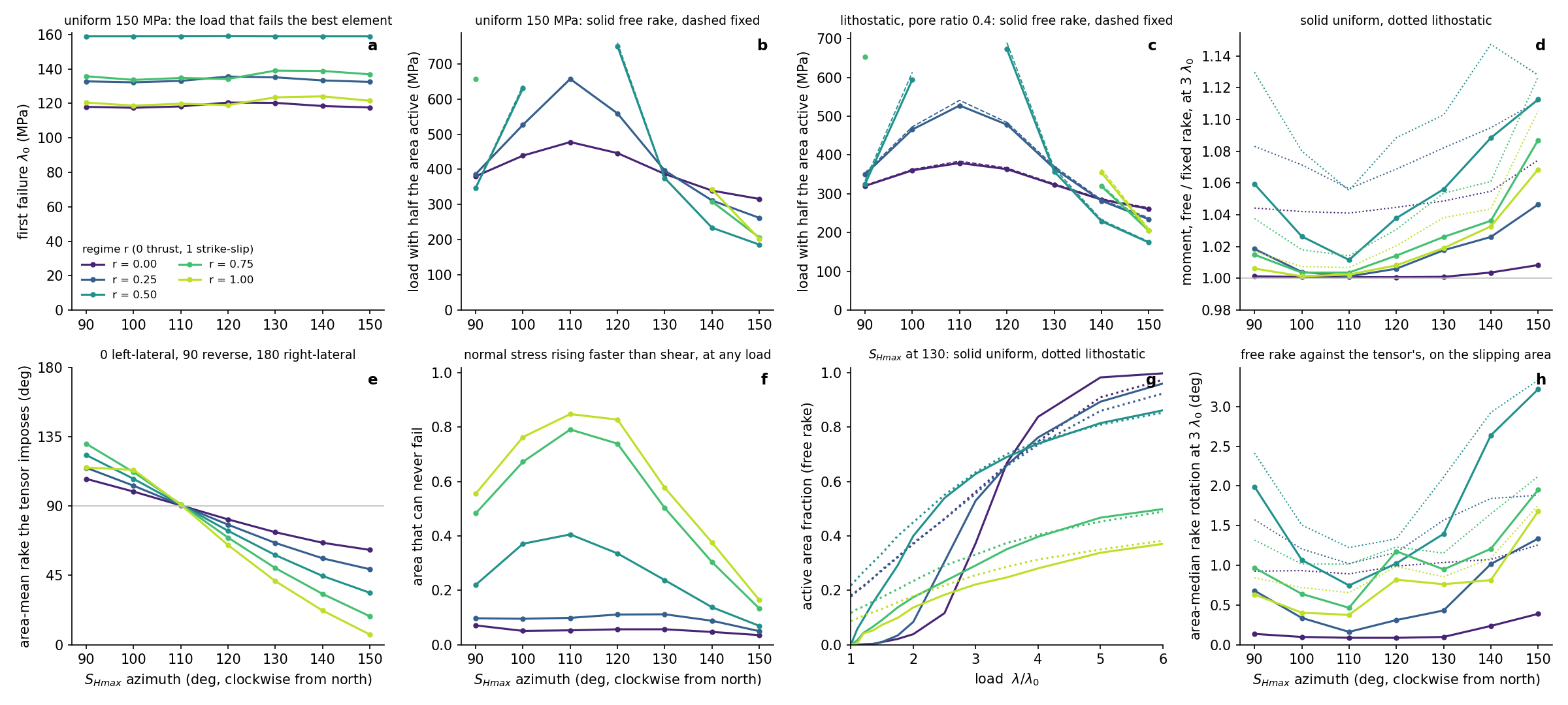
The first failure says nothing about the tensor. λ0 is 117 to 159 MPa and flat in azimuth (panel a): it is set by whichever sliver of the supplied mesh happens to be best oriented, and it moves with the regime only because the family’s intermediate stress changes the normal stress on that sliver. The load at which half the fault is slipping (b, c) is the number that discriminates.
Fault-normal compression is the hardest way to load this fault. With the compressive axis at 110°, normal to the strike, the thrust tensor needs 478 MPa of maximum shear to bring half the area to failure under either rule, against 387 MPa at 130° and 316 MPa at 150°: a 60° fault is poorly oriented for pure thrust, and obliquity helps. For the strike-slip half of the family the fault-normal case does not activate at all: with r ≥ 0.5 at 100° to 120°, a third to 85 % of the area has its normal stress rising faster than its shear and can never fail (e), and half the area is not slipping by 6 λ0. The same tensors at 150° are the easiest in the sweep, 186 to 203 MPa, two and a half times less than fault-normal thrust.
The observed sense of slip picks the oblique thrust-like corner. The fault is reverse with a left-lateral component. In this family that rake, 45° to 75°, appears only with the compressive axis at 120° to 150° (d), and near the plate-convergence azimuth of about 130° only the thrust-like half of the family (r ≤ 0.5) brings half the fault to failure within the scan, at 377 to 397 MPa, with a mean rake of 58° to 73°. The tensors that both load the fault and slip it the right way are therefore the oblique, thrust-leaning ones, and the pure strike-slip tensor at the convergence azimuth clamps half of the fault shut.
The strength profile shifts the numbers, not the ordering. The lithostatic model, weak in its shallow rows, has 3 to 45 % of the area slipping already at the uniform model’s first failure and reaches half the area at loads up to 20 % lower for the thrust-like tensors and within 5 % for the strike-slip ones (c against b), with a smoother activation curve (f); every ranking of azimuth and regime is the same. The area the load drives into tension stays under 0.2 % on the uniform model and under 1.2 % on the lithostatic one at 6 λ0, so the linear criterion is not being used where it is wrong.
The free rake moves the moment, not the map. Letting the slip turn changes the load at which half the fault is active by under 2 % on every tensor (b, c, solid against dashed), switches on a few elements and switches none off, and reverses the sense of slip on at most a handful of slivers whose neighbours turn their shear round. What it changes is the moment (d): by 0.1 % for pure thrust at any azimuth, and by up to 11 % on the uniform model and 15 % on the lithostatic one at r = 0.5 and the oblique azimuths, where the regional shear on the fault is smallest against what the slipping neighbours add and the tensor itself is ambiguous between reverse and sinistral. The slip turns by an area-median 0.1° to 0.4° for thrust and 1° to 3° for the strike-slip and axial tensors at 3 λ0 (h), with a 90th percentile under 10°. The fixed rake is therefore a sub-percent approximation where the tensor is thrust-like and a several-percent one where it is not, and the maps under either rule tell the same story.
The kernel does not matter here, and the slivers did not break the solve. Under either rule the classical dislocation and the mollified kernel put the half-active load within 1.4 % of each other on every tensor, the active fraction within 0.011 at every load, and the moment within 4 % at the median. The uniqueness indicator for the collocation kernels is the smallest eigenvalue of the symmetric part of the area-weighted operator, as a fraction of its median eigenvalue: it is positive on all 35 tensors for both, +0.0007 to +0.0009 for the mollified kernel and +0.03 to +0.08 for the classical one, the small values being the fault’s softest mode, slip of the whole 100 km surface at once, against the element-scale median. So the uniqueness hypothesis holds here for every kernel, and the projected Gauss–Seidel sweeps converged in all 5,460 solves, scalar and cone alike, without the active-set fallback. The slips themselves, tens of metres at three times the first failure, are what a static load of several hundred MPa produces on a frictional surface with no other faults to share it: read the maps for where slip goes, not for how much.
The Galerkin kernel draws the same map with less slip, and it is the one with a proof. Its area-weighted operator is positive definite on all 35 tensors (smallest eigenvalue +0.0004 to +0.0006 of the median, the same whole-fault mode), so each of its 1,820 solves has one solution by theorem and the sweeps converge by theorem; they did, with no fallback. It puts the half-active load within 2.1 % of the mollified collocation kernel on every tensor (median 0.6 % lower) and the active fraction within 0.013 at every load, under either rule: the same elements slip. Each slips a little less, so the moment is 7 % lower at the median and between 0 and 17 % lower across the sweep, in the same proportion at every depth, because averaging the self-traction over an element reads it higher than the centroid does. The same operator is 3 % softer than collocation on the gate’s penny; here, with the supplied 0.12 km slivers at the same mollification width, the gap is twice that. The map is the robust product and the moment the fragile one, on every kernel.
What this is not
- Not a model of Taiwan: one fault, with none of the others and none of the plate interface, so there is no interaction and no shadow.
- Not a slip-rate model: the load is a static stress and the answer a static slip, with no time, no geodesy and no geologic rate fitted.
- Not an absolute stress: everything is quoted relative to the tensor’s own first failure or in MPa of maximum shear, and the 150 MPa and the pore ratio are assumptions, not measurements.
- Not a converged mesh: the segments are used as supplied, at one resolution, with their slivers.
- Uniform friction, and no coupling of the normal stress to slip in either rule, which is where genuine Coulomb non-uniqueness would enter. Opening is not modelled; where the load drives the normal stress through zero the linear criterion is wrong and the manifest says where.
Reproducing it
python studies/active_fractal/selfcheck.py -k taiwan    # the inputs
python studies/active_fractal/selfcheck.py -k rake      # the free-rake solver on a penny
python studies/active_fractal/selfcheck.py -k galerkin  # the symmetric form of the kernel
python studies/active_fractal/taiwan.py assemble --workers 8                   # the folded matrix, cached
python studies/active_fractal/taiwan.py assemble --workers 8 --form galerkin   # its Galerkin form, 9 points per element
python studies/active_fractal/taiwan.py run                    # 70 tensors x 3 kernels x 2 rules x 13 loads
python studies/active_fractal/taiwan.py figure                 # website/src/figures/taiwan_sweep.png
python studies/active_fractal/taiwan.py payload                # website/public/data/taiwan_*